First time studying this topic?

Launch the interactive walkthrough to discover each component, including the 3D Q-Sphere Lab & Python in Colab.

Topic 5.1

Why Learn Quantum Computing? The Post-Moore Era

Understand the exponential computational limits of classical silicon and why quantum computing is the next grand paradigm.

Learning Objectives

✓Analyze the physical breakdown of Moore’s Law at atomic silicon scales
✓Understand why classical supercomputers cannot simulate nature and chemistry
✓Examine how quantum mechanics unlocks exponential state spaces ($2^n$)

📖Let's Begin with a Story

In 1981, legendary Nobel laureate physicist Richard Feynman gave a keynote address at MIT titled "Simulating Physics with Computers." Feynman posed a fundamental paradox: If you want to simulate a simple caffeine molecule (

C_8 H_{10} N_4 O_2

), you have to track the quantum wavefunctions and electron configurations of just 24 atoms. To represent that quantum state on a classical supercomputer would require more memory bits than there are grains of sand on the entire planet Earth. For a penicillin molecule, it would require more bits than there are subatomic particles in the observable universe. Feynman concluded with one of the most famous quotes in modern science: "Nature isn't classical, dammit, and if you want to make a simulation of nature, you'd better make it quantum mechanical, and by golly it's a wonderful problem, because it doesn't look so easy."

Why Does Mastering This Matter in Practice?

🎯 Practical & Engineering Stakes

The next technological revolution

Classical computing is hitting physical quantum tunneling limits in silicon chips. Quantum computing is not just a faster processor; it is an entirely new mathematical model of computation that solves previously impossible problems in drug discovery, materials science, and cryptography.

🎮 Fun Learning Zone

Grasp complex quantum concepts visually with zero prior physics or math knowledge!

Zero Prerequisites

Visual Concept Storyboard

The Atomic Traffic Jam & The Magic Water Wave

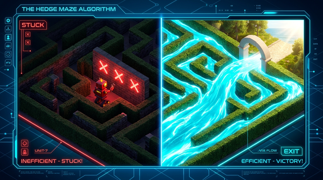
High-Fidelity Analogy Visualization

Visual contrast capturing the paradigm shift without needing to read the full text.

Classical: Serial / ConstrainedQuantum: Coherent Wave Parallelism

Visual takeaway: Understand in 5 seconds

Everyday Analogy: The Atomic Traffic Jam & The Magic Water Wave

Imagine you are driving in a city where cars get smaller every year. First they are big buses, then compact cars, then roller skates. Eventually, the cars are shrunk down to single atoms! At this atomic scale, silicon walls are so paper-thin that electrons literally leak through them like ghosts walking through walls (quantum tunneling). Transistors cannot be made any smaller without breaking physics! But while classical computers are like single cars trying every street in a giant maze one-by-one, a quantum computer behaves like an ocean wave flooding into the maze: it explores every route simultaneously!

🧪

Interactive Mental Sandbox

Try It Yourself

Hedge Maze Corridor Challenge

Escape a maze with 1,000 corridors and only 1 exit.

Click "Run Classical Robot" or "Unleash Quantum Wave" to test escape dynamics!

📖 The Thought Experiment Prompt:“Close your eyes and try this mental experiment: You are locked in a hedge maze with 1,000 corridors, and only one exit. If you are a classical robot, you must walk down Path 1, hit a wall, backtrack, walk down Path 2, hit a wall... taking hours. Now imagine turning into a tidal wave of water: you pour into the entrance, rush down all 1,000 corridors in the exact same millisecond, and wash out the exit immediately! That is why we learn quantum: it turns serial guessing into simultaneous wave dynamics.”

✨ The "Aha!" Moment

Classical silicon chips are hitting an absolute atomic wall (the end of Moore’s Law). Quantum computing does not just make computers faster; it replaces mechanical rock-pushing with nature’s native wave mechanics!

What Is It?

Simple Explanation

Classical computers are like a person trying to escape a giant hedge maze by walking down every path one by one. If they hit a dead end, they backtrack and try the next path. A quantum computer is like a wave of water flooding into the maze all at once. It flows through all paths simultaneously, cancels out the wrong dead ends through interference, and reveals the exit instantly!

Technical Explanation

Classical digital computers represent information as binary states in a discrete Boolean algebra

\{0, 1\}^n

. Quantum computers exploit quantum mechanical phenomena—specifically coherent superposition in complex Hilbert spaces

\mathcal{H} = \mathbb{C}^{2^n}

and non-local entanglement—enabling algorithms with polynomial complexity

\mathcal{O}(\text{poly}(n))

for problems in bounded-error quantum polynomial time (BQP) that are intractable in classical complexity class BPP.

📚 Key Terms

Moore’s Law

Simple: The rule that computer chips doubled in power every two years, which is now hitting physical atomic limits.

Technical: Empirical observation by Gordon Moore (1965) that transistor density on integrated circuits doubles approximately every 18–24 months.

Quantum Supremacy / Advantage

Simple: The historic moment when a quantum computer performs a calculation that no classical supercomputer on Earth could complete in a reasonable time.

Technical: Demonstration of a programmable quantum device solving a well-defined computational problem substantially faster than the classical state of the art.

Hilbert Space

Simple: The mathematical universe where quantum wavefunctions live.

Technical: A complete complex inner product vector space

\mathbb{C}^d

hosting quantum state vectors.

Q-Sphere Lab: Why Learn Quantum Computing? The Post-Moore Era

IBM Q-Sphere Model

Interactive 3D state vector exploration, unitary transformation gates, and Born rule collapse for Topic 5.1

Azimuth: 45°Elevation: 25°(Click & drag sphere to orbit)

Q-Sphere Phase Color:

0 π/2 π 3π/2

Quantum Statevector

dim(H) = 2

|ψ⟩ = (1.000 + 0.000i)|0⟩
+ (0.000 + 0.000i)|1⟩

Polar Angle (θ):0.0° (0.000π rad)

Phase Angle (ϕ):0.0° (0.000π rad)

Born Rule Probabilities: P(x) = |⟨x|ψ⟩|²Σ P = 1.00

P(|0⟩) = |α|²100.0%

P(|1⟩) = |β|²0.0%

Quantum Measurement

Apply Single-Qubit Unitary Gates

Presets:

Continuous Polar Angle θ (0° = |0⟩, 180° = |1⟩):0.0°

Continuous Phase Angle ϕ (0° to 360°):0.0°

Recent Operations Log:

#1Initial state: |0⟩

📐 Mathematical Foundation

LaTeX KaTeX

\dim(\mathcal{H}) = 2^n

What does it mean?

Exponential Dimensionality of Quantum State Space: Adding just ONE physical qubit (

n+1

) doubles the entire mathematical capacity of the quantum computer (

2 \times 2 \times 2...

), creating an astronomical state space that classical supercomputers can never simulate.

Understanding the Symbols

Symbol / Term	Meaning	Beginner Interpretation
$n$	Number of physical qubits	Number of quantum particles (e.g., electrons, trapped ions) in the processor
$2^n$	Number of simultaneous basis states	Total parallel slots/realities held in superposition at once
$\dim(\mathcal{H})$	Dimension of Hilbert state space	The size of the mathematical universe housing the quantum wave

📊 Numerical Example

Comparing simultaneous states and classical RAM needed to simulate n qubits:

• n = 1 qubit: 2^1 = 2 states (Spin Down and Spin Up) • n = 3 qubits: 2^3 = 2 × 2 × 2 = 8 simultaneous states • n = 10 qubits: 2^10 = 1,024 states (requires ~16 KB RAM) • n = 50 qubits: 2^50 ≈ 1.125 × 10^15 states (requires ~18 Petabytes of RAM!) • n = 300 qubits: 2^300 ≈ 2.03 × 10^90 states

Result: At 300 qubits, 2^300 exceeds all 10^80 atoms in the observable universe. Classical supercomputers hit an absolute mathematical wall.

⚙️ How Does It Work?

State Initialization

Initialize n qubits into ground state |00...0>.

Superposition Creation

Apply Hadamard gates to put system into simultaneous superposition of all 2^n states.

Quantum Interference

Apply unitary transformations that constructively amplify correct answers and destructively cancel incorrect paths.

Measurement Collapse

Read out classical bit string revealing the optimal solution with high probability.

🌍 Where Is It Used?

Nitrogen Fixation & Fertilizer Catalyst

Problem: Manufacturing fertilizer uses 2% of the entire world’s energy supply (Haber-Bosch process). Bacteria do this at room temperature using a nitrogenase enzyme, but classical computers cannot simulate its electron structure.

Solution: Quantum computers will model the active FeMo-cofactor, designing room-temperature chemical catalysts.

Battery Chemistry Simulation

Problem: Developing solid-state lithium electrolytes for electric vehicles takes decades of wet lab trial and error.

Solution: Quantum chemistry algorithms simulate cathode crystal lattice bonding directly.

🎯 Try It Yourself

How many classical complex numbers are required to describe the exact state of a 10-qubit quantum computer?

Interactive activity component

🐍 Python Hands-On: Simulating Exponential State Space Scaling in Qiskit

Construct an n-qubit superposition state with Qiskit and analyze how Hilbert state space explodes exponentially.

Open Colab

1Install Required Packages

For Google Colab or Jupyter notebooks, run this shell command to install the required dependencies:

Terminal / Notebook Install Commandbash

!pip install qiskit qiskit-aer numpy

Packages:

qiskitqiskit-aernumpy

2Import Libraries

Import Statementspython

1 from qiskit import QuantumCircuit
2 from qiskit.quantum_info import Statevector
3 import numpy as np

from qiskit import QuantumCircuit → Qiskit class to build quantum circuits

from qiskit.quantum_info import Statevector → Simulates exact quantum statevectors

import numpy as np → Numerical analysis of state space dimensions

3Demonstration Code & Logic

Python Execution Codepython

1 # 1. Build a 3-qubit circuit in equal superposition
2 qc = QuantumCircuit(3)
3 qc.h(range(3))
4 sv = Statevector.from_instruction(qc)
5 print(f'3-Qubit Circuit Statevector dimension: {sv.dim}')
6 print('Amplitudes for |000> through |111>:')
7 for idx, amp in enumerate(sv.data):
8     print(f'  |{idx:03b}> : {amp.real:.4f} + {amp.imag:.4f}j')
9  
10 # 2. Classical RAM requirement calculation for n qubits
11 print('\nScaling Analysis: Why Classical Supercomputers Fail:')
12 for n in [10, 20, 30, 40, 50]:
13     states = 2**n
14     ram_bytes = states * 16  # 16 bytes per complex128 number
15     ram_gb = ram_bytes / (1024**3)
16     if ram_gb < 1024:
17         ram_str = f'{ram_gb:.4f} GB'
18     elif ram_gb < 1024**2:
19         ram_str = f'{ram_gb / 1024:.2f} TB'
20     else:
21         ram_str = f'{ram_gb / (1024**2):.2f} Petabytes (PB)'
22     print(f'  {n:2d} Qubits -> {states:16,d} Amplitudes -> {ram_str}')

Step-by-Step Code Breakdown:

# 1. Build a 3-qubit circuit in equal superposition

Create circuit with 3 qubits

qc = QuantumCircuit(3)

Allocate 3 qubits in ground state |000>

qc.h(range(3))

Apply Hadamard gate to all 3 qubits simultaneously

sv = Statevector.from_instruction(qc)

Simulate exact statevector

print(f'3-Qubit Circuit Statevector dimension: {sv.dim}')

Display dimension 2^3 = 8

print('Amplitudes for |000> through |111>:')

Label

for idx, amp in enumerate(sv.data):

Loop amplitudes

print(f' |{idx:03b}> : {amp.real:.4f} + {amp.imag:.4f}j')

Display amplitudes (1/sqrt(8) = 0.3536)

# 2. Classical RAM requirement calculation for n qubits

Exponential scaling

print('\nScaling Analysis: Why Classical Supercomputers Fail:')

Header

for n in [10, 20, 30, 40, 50]:

Qubit milestones

states = 2**n

Total complex amplitudes required

ram_bytes = states * 16 # 16 bytes per complex128 number

Memory demand

ram_gb = ram_bytes / (1024**3)

Convert to GB

if ram_gb < 1024:

ram_str = f'{ram_gb:.4f} GB'

elif ram_gb < 1024**2:

ram_str = f'{ram_gb / 1024:.2f} TB'

else:

ram_str = f'{ram_gb / (1024**2):.2f} Petabytes (PB)'

print(f' {n:2d} Qubits -> {states:16,d} Amplitudes -> {ram_str}')

Print scaling

📋 Complete Script (All-in-One)

Click "Copy for Colab", open Google Colab, paste into a single cell, and run.

Google Colab Notebook Scriptpython

1 # =========================================================
2 # Simulating Exponential State Space Scaling in Qiskit
3 # Prepared for Google Colab (Run with Shift + Enter)
4 # =========================================================
5  
6 # Step 1: Install required packages
7 !pip install qiskit qiskit-aer numpy
8  
9 # Step 2: Import libraries
10 from qiskit import QuantumCircuit
11 from qiskit.quantum_info import Statevector
12 import numpy as np
13  
14 # Step 3: Run Demonstration
15 # 1. Build a 3-qubit circuit in equal superposition
16 qc = QuantumCircuit(3)
17 qc.h(range(3))
18 sv = Statevector.from_instruction(qc)
19 print(f'3-Qubit Circuit Statevector dimension: {sv.dim}')
20 print('Amplitudes for |000> through |111>:')
21 for idx, amp in enumerate(sv.data):
22     print(f'  |{idx:03b}> : {amp.real:.4f} + {amp.imag:.4f}j')
23  
24 # 2. Classical RAM requirement calculation for n qubits
25 print('\nScaling Analysis: Why Classical Supercomputers Fail:')
26 for n in [10, 20, 30, 40, 50]:
27     states = 2**n
28     ram_bytes = states * 16  # 16 bytes per complex128 number
29     ram_gb = ram_bytes / (1024**3)
30     if ram_gb < 1024:
31         ram_str = f'{ram_gb:.4f} GB'
32     elif ram_gb < 1024**2:
33         ram_str = f'{ram_gb / 1024:.2f} TB'
34     else:
35         ram_str = f'{ram_gb / (1024**2):.2f} Petabytes (PB)'
36     print(f'  {n:2d} Qubits -> {states:16,d} Amplitudes -> {ram_str}')

⚡ How to Run in Google Colab (3 Quick Steps)

Click "Copy for Google Colab" above.
Click Open New Google Colab Notebook (opens in a new tab).
Click on the first empty code cell, press Ctrl + V (or Cmd + V) to paste, then press Shift + Enter to execute!

Launch Blank Colab Notebook

🔄 Algorithmic Execution Flow

Create Qiskit Circuit

Allocate 3 qubits and apply Hadamard gates to create full superposition.

→

Extract Statevector

Use Qiskit Statevector to inspect exact complex probability amplitudes.

→

Calculate Memory Explosion

Demonstrate why 50 qubits requires 16 Petabytes of RAM, creating the physical foundation for quantum advantage.

📥 Input / Initial State

Qiskit QuantumCircuit(3) with H gates applied to all wires.

📤 Expected Output

3-Qubit Circuit Statevector dimension: 8
Amplitudes for |000> through |111>: 0.3536 each
10 Qubits -> 1,024 Amplitudes (0.000015 GB)
30 Qubits -> 1,073,741,824 Amplitudes (16.00 GB)
50 Qubits -> 1.12 x 10^15 Amplitudes (16.00 Petabytes)

💡 What Does This Demonstration Show?

In Qiskit, each added qubit doubles the Hilbert space dimension (2^n). At 50 qubits, holding the state vector classically requires 16 Petabytes of RAM, demonstrating why quantum hardware provides an exponential computational advantage.

Course Learning Resource • Slide Deck19 Slides

Comprehensive Foundation in Quantum Computing

From Probability and Complex Numbers to Qubits, Interference, Entanglement, and Multi-Qubit Systems by Dr. Syed Muzamil Basha.

Author: Dr. Syed Muzamil Basha• FDP Approved Curriculum

Open in New Tab

Available Slide Decks:

📝 Learning Check

Test your understanding with these questions. Remember, this is for learning, not examination!

Question 1: Why did Richard Feynman propose building quantum computers in 1981?

Question 2: What is the dimensionality of the Hilbert space for a 50-qubit quantum computer?

Question 3: What fundamental physical limit is causing Moore's Law to break down in silicon transistors?

Question 4: Which complexity class contains problems solvable efficiently on quantum computers but believed intractable classically?

Question 5: How many complex numbers are required to classically simulate the quantum state of a caffeine molecule (24 atoms, 102 electrons)?

Previous: Deep Q-Networks (DQN): Module 4 Capstone Next: History of Quantum Computing: From Theory to Silicon

1	from qiskit import QuantumCircuit
2	from qiskit.quantum_info import Statevector
3	import numpy as np

1	# =========================================================
2	# Simulating Exponential State Space Scaling in Qiskit
3	# Prepared for Google Colab (Run with Shift + Enter)
4	# =========================================================
5
6	# Step 1: Install required packages
7	!pip install qiskit qiskit-aer numpy
8
9	# Step 2: Import libraries
10	from qiskit import QuantumCircuit
11	from qiskit.quantum_info import Statevector
12	import numpy as np
13
14	# Step 3: Run Demonstration
15	# 1. Build a 3-qubit circuit in equal superposition
16	qc = QuantumCircuit(3)
17	qc.h(range(3))
18	sv = Statevector.from_instruction(qc)
19	print(f'3-Qubit Circuit Statevector dimension: {sv.dim}')
20	print('Amplitudes for \|000> through \|111>:')
21	for idx, amp in enumerate(sv.data):
22	print(f' \|{idx:03b}> : {amp.real:.4f} + {amp.imag:.4f}j')
23
24	# 2. Classical RAM requirement calculation for n qubits
25	print('\nScaling Analysis: Why Classical Supercomputers Fail:')
26	for n in [10, 20, 30, 40, 50]:
27	states = 2**n
28	ram_bytes = states * 16 # 16 bytes per complex128 number
29	ram_gb = ram_bytes / (1024**3)
30	if ram_gb < 1024:
31	ram_str = f'{ram_gb:.4f} GB'
32	elif ram_gb < 1024**2:
33	ram_str = f'{ram_gb / 1024:.2f} TB'
34	else:
35	ram_str = f'{ram_gb / (1024**2):.2f} Petabytes (PB)'
36	print(f' {n:2d} Qubits -> {states:16,d} Amplitudes -> {ram_str}')