First time studying this topic?

Launch the interactive walkthrough to discover each component, including the 3D Q-Sphere Lab & Python in Colab.

Topic 5.2

History of Quantum Computing: From Theory to Silicon

Trace the lineage of quantum information: from Planck and Einstein to Feynman, Deutsch, Shor, Grover, and modern noisy intermediate-scale quantum (NISQ) devices.

Learning Objectives

✓Chronicle key theoretical milestones (Feynman, Benioff, Deutsch)
✓Understand the seismic impact of Shor’s Algorithm (1994) and Grover’s Search (1996)
✓Survey modern physical implementations: Superconducting circuits, Trapped Ions, Photonic, and Silicon spin qubits

📖Let's Begin with a Story

In 1994, an applied mathematician at Bell Laboratories named Peter Shor published an algorithm that sent a shiver through the global intelligence and banking communities. Shor proved that a sufficiently large quantum computer could factor large composite integers in polynomial time (

O((\log N)^3)

). Virtually all modern global cybersecurity—including RSA public-key encryption, HTTPS internet banking, and encrypted military transmissions—relies on the assumption that factoring a 2048-bit integer would take the fastest classical supercomputers billions of years. Shor's algorithm proved that a quantum computer could break that encryption in a few hours. Overnight, quantum computing transformed from an academic curiosity into a multibillion-dollar global geopolitical race.

Why Should You Learn History of Quantum Computing: From Theory to Silicon?

🎯 Practical & Engineering Stakes

The historical arc

Understanding how quantum computing evolved from thought experiments to cloud-accessible physical QPUs helps you appreciate current technological roadblocks and future breakthroughs.

🎮 Fun Learning Zone

Grasp complex quantum concepts visually with zero prior physics or math knowledge!

Zero Prerequisites

Visual Concept Storyboard

The Renaissance Clockmaker vs. Nature’s Secret Code

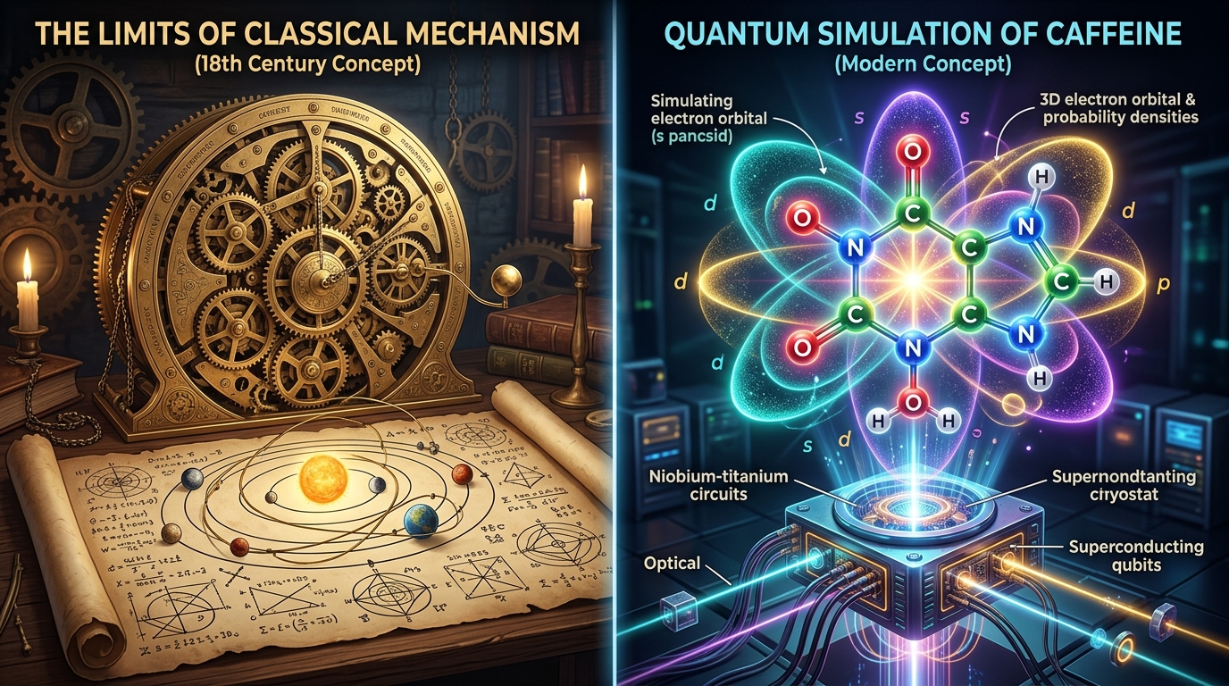
High-Fidelity Analogy Visualization

Visual contrast capturing the paradigm shift without needing to read the full text.

Classical: Serial / ConstrainedQuantum: Coherent Wave Parallelism

Visual takeaway: Understand in 5 seconds

Everyday Analogy: The Renaissance Clockmaker vs. Nature’s Secret Code

For centuries, astronomers tried to map planetary orbits using complicated gears and circles on flat paper (Ptolemy’s epicycles). The math was a nightmare because the planets were moving in 3D ellipses around the sun! In 1981, physicist Richard Feynman pointed out that computer scientists were doing the exact same silly thing: trying to simulate 3D quantum nature using flat classical 1s and 0s. Feynman said: If you want to simulate nature, your machine itself had better be quantum mechanical!

🧪

Interactive Mental Sandbox

Try It Yourself

Feynman's Molecule State Space Calculator

Simulate why a 1-cup caffeine molecule breaks classical computers.

N = 24 Qubits / Atoms

Number of Simulated Atoms: 242^24 states

Quantum Hilbert Dimension ($2^N$):16,777,216

💡 Milestone: ☕ Caffeine Molecule (24 atoms): Exceeds all grains of sand on Earth (~7.5 × 10¹⁸ bits)!

Yet a warm cup of coffee calculates all 24 caffeine atom wavefunctions effortlessly in femtoseconds because nature runs quantum mechanics natively!

📖 The Thought Experiment Prompt:“Picture holding a single cup of coffee containing caffeine molecules ($C_8 H_{10} N_4 O_2$). It contains just 24 atoms. Try to write down all the electron interactions on classical hard drives: you would need more memory bits than all the grains of sand on every beach on planet Earth! Yet the coffee cup in your hand calculates those interactions effortlessly in real-time. That realization sparked the entire 40-year revolution of quantum computing from Feynman, Deutsch, and Shor to today.”

✨ The "Aha!" Moment

Quantum computing was not created to make spreadsheets faster; it was born because classical mathematics physically cannot simulate atomic nature and chemistry!

What Is It?

Simple Explanation

The story of quantum computing in 4 acts: 1. 1900-1930s (Physics): Einstein, Bohr, and Schrödinger discover that atoms follow strange quantum rules. 2. 1980s (The Dream): Feynman and David Deutsch realize we can build computers that use these quantum rules. 3. 1990s (The Proof): Peter Shor and Lov Grover invent algorithms proving quantum computers can crack codes and search databases at blinding speed. 4. Today (Hardware): Tech giants and startups build real physical quantum chips in sub-zero dilution refrigerators!

Technical Explanation

Key historical milestones: - 1980 (Paul Benioff): Showed quantum mechanical Turing machines are thermodynamically possible. - 1985 (David Deutsch): Formulated the Universal Quantum Turing Machine and first quantum algorithm. - 1994 (Peter Shor): Polynomial-time prime factorization algorithm. - 1996 (Lov Grover):

O(\sqrt{N})

quadratic database search algorithm. - 2019 (Google Quantum AI): Sycamore 53-qubit processor demonstrates quantum computational supremacy on random circuit sampling.

📚 Key Terms

Shor’s Algorithm

Simple: The famous quantum algorithm that can crack modern internet encryption (RSA) by factoring large numbers quickly.

Technical: Polynomial-time quantum algorithm for integer factorization and discrete logarithms using Quantum Fourier Transform.

NISQ Era

Simple: Noisy Intermediate-Scale Quantum: our current era of 50-1,000 qubit machines that are powerful but prone to noise and errors.

Technical: Current computational epoch characterized by 50–1000 noisy physical qubits without fault-tolerant quantum error correction (John Preskill, 2018).

Q-Sphere Lab: History of Quantum Computing: From Theory to Silicon

IBM Q-Sphere Model

Interactive 3D state vector exploration, unitary transformation gates, and Born rule collapse for Topic 5.2

Azimuth: 45°Elevation: 25°(Click & drag sphere to orbit)

Q-Sphere Phase Color:

0 π/2 π 3π/2

Quantum Statevector

dim(H) = 2

|ψ⟩ = (1.000 + 0.000i)|0⟩
+ (0.000 + 0.000i)|1⟩

Polar Angle (θ):0.0° (0.000π rad)

Phase Angle (ϕ):0.0° (0.000π rad)

Born Rule Probabilities: P(x) = |⟨x|ψ⟩|²Σ P = 1.00

P(|0⟩) = |α|²100.0%

P(|1⟩) = |β|²0.0%

Quantum Measurement

Apply Single-Qubit Unitary Gates

Presets:

Continuous Polar Angle θ (0° = |0⟩, 180° = |1⟩):0.0°

Continuous Phase Angle ϕ (0° to 360°):0.0°

Recent Operations Log:

#1Initial state: |0⟩

📐 Mathematical Foundation

LaTeX KaTeX

N_{\text{eval, classical}} = 2 \quad \text{vs} \quad N_{\text{eval, quantum}} = 1

What does it mean?

Deutsch's Query Complexity Theorem (1985): Proves that a quantum computer can determine whether an unknown black-box function f(x) is constant or balanced in just ONE single query, whereas any classical computer on Earth mathematically requires TWO queries.

Understanding the Symbols

Symbol / Term	Meaning	Beginner Interpretation
$f(x)$	Black-box function (Oracle)	A mystery computer program that maps input bit x ∈ {0, 1} to an output bit
$N_{\text{eval}}$	Number of function evaluations	Number of queries or calls made to the mystery function
$N_{\text{eval, classical}} = 2$	Classical query requirement	Must evaluate f(0), then evaluate f(1), and compare them
$N_{\text{eval, quantum}} = 1$	Quantum query requirement	Evaluates global property $f(0) \oplus f(1)$ in a single shot using superposition

📊 Numerical Example

Testing if a coin-toss black-box is fair (balanced) or rigged (constant):

Classical Evaluation: Step 1: Query x = 0 → f(0) = 1 (Outcome uncertain, answer still unknown!) Step 2: Query x = 1 → f(1) = 1 (Total: 2 evaluations needed to determine constant) Quantum Evaluation (Deutsch Algorithm): Step 1: Prepare input state

|\psi\rangle

= (

|0\rangle

|1\rangle

)/√2 Step 2: Query Oracle once with phase kickback: (-1)^{f(x)} Step 3: Measure first qubit: 0 indicates Constant, 1 indicates Balanced!

Result: The global property is unlocked in 1 quantum step vs 2 classical steps (50% reduction in query complexity).

⚙️ How Does It Work?

Theoretical Foundation (1980s)

Deutsch proves quantum parallelism using unitary quantum gates.

Algorithmic Speedup (1990s)

Shor and Grover prove exponential and polynomial advantages over classical computing.

Physical Realization (2000s-Present)

Superconducting transmon qubits and trapped ytterbium ions transition from physics labs to cloud APIs.

🌍 Where Is It Used?

Post-Quantum Cryptography (PQC)

Problem: NIST must standardize new encryption algorithms before fault-tolerant quantum computers break RSA.

Solution: Lattice-based cryptography algorithms (Kyber, Dilithium) replace factoring-based public key infrastructure.

🎯 Try It Yourself

Which quantum algorithm, discovered in 1994, proved that quantum computers could break RSA public-key encryption in polynomial time?

Interactive activity component

🐍 Python Hands-On: Executing Deutsch's Historic Quantum Algorithm (1985) in Qiskit

Build and run David Deutsch's landmark 1985 quantum algorithm to determine if a Boolean function is constant or balanced in a single evaluation.

Open Colab

1Install Required Packages

For Google Colab or Jupyter notebooks, run this shell command to install the required dependencies:

Terminal / Notebook Install Commandbash

!pip install qiskit qiskit-aer

Packages:

qiskitqiskit-aer

2Import Libraries

Import Statementspython

1 from qiskit import QuantumCircuit
2 from qiskit.quantum_info import Statevector

from qiskit import QuantumCircuit → Qiskit circuit constructor

from qiskit.quantum_info import Statevector → Statevector simulator

3Demonstration Code & Logic

Python Execution Codepython

1 # Deutsch Algorithm: Determine if f(x) is constant or balanced in 1 query
2 # Let f(x) be a balanced function: f(0)=0, f(1)=1 (implemented via CNOT)
3 qc = QuantumCircuit(2, 1)
4 # Step 1: Initialize ancilla to |1> and apply Hadamard to both qubits
5 qc.x(1)
6 qc.h([0, 1])
7 # Step 2: Query the quantum oracle (CNOT implements balanced f(x)=x)
8 qc.cx(0, 1)
9 # Step 3: Interference on input qubit
10 qc.h(0)
11 qc.measure(0, 0)
12 print('Deutsch Algorithm Circuit Diagram in Qiskit:')
13 print(qc.draw('text'))
14 sv = Statevector.from_instruction(qc.remove_final_measurements(inplace=False))
15 print('\nFinal State Vector:', sv.data.round(3))
16 print('Result: Measuring qubit 0 yields 1, proving f(x) is BALANCED in 1 query!')

Step-by-Step Code Breakdown:

# Deutsch Algorithm: Determine if f(x) is constant or balanced in 1 query

Setup

# Let f(x) be a balanced function: f(0)=0, f(1)=1 (implemented via CNOT)

Oracle definition

qc = QuantumCircuit(2, 1)

2 qubits: q0=input, q1=ancilla; 1 classical bit

# Step 1: Initialize ancilla to |1> and apply Hadamard to both qubits

Superposition prep

qc.x(1)

Put ancilla in |1>

qc.h([0, 1])

Create state |+>|->

# Step 2: Query the quantum oracle (CNOT implements balanced f(x)=x)

Oracle query

qc.cx(0, 1)

Phase kickback from target |-> into control |+>

# Step 3: Interference on input qubit

Interference

qc.h(0)

Interference transforms |- > into |1> for balanced function

qc.measure(0, 0)

Measure input qubit

print('Deutsch Algorithm Circuit Diagram in Qiskit:')

print(qc.draw('text'))

Draw circuit ASCII

sv = Statevector.from_instruction(qc.remove_final_measurements(inplace=False))

Analyze

print('\nFinal State Vector:', sv.data.round(3))

State

print('Result: Measuring qubit 0 yields 1, proving f(x) is BALANCED in 1 query!')

Conclusion

📋 Complete Script (All-in-One)

Click "Copy for Colab", open Google Colab, paste into a single cell, and run.

Google Colab Notebook Scriptpython

1 # =========================================================
2 # Executing Deutsch's Historic Quantum Algorithm (1985) in Qiskit
3 # Prepared for Google Colab (Run with Shift + Enter)
4 # =========================================================
5  
6 # Step 1: Install required packages
7 !pip install qiskit qiskit-aer
8  
9 # Step 2: Import libraries
10 from qiskit import QuantumCircuit
11 from qiskit.quantum_info import Statevector
12  
13 # Step 3: Run Demonstration
14 # Deutsch Algorithm: Determine if f(x) is constant or balanced in 1 query
15 # Let f(x) be a balanced function: f(0)=0, f(1)=1 (implemented via CNOT)
16 qc = QuantumCircuit(2, 1)
17 # Step 1: Initialize ancilla to |1> and apply Hadamard to both qubits
18 qc.x(1)
19 qc.h([0, 1])
20 # Step 2: Query the quantum oracle (CNOT implements balanced f(x)=x)
21 qc.cx(0, 1)
22 # Step 3: Interference on input qubit
23 qc.h(0)
24 qc.measure(0, 0)
25 print('Deutsch Algorithm Circuit Diagram in Qiskit:')
26 print(qc.draw('text'))
27 sv = Statevector.from_instruction(qc.remove_final_measurements(inplace=False))
28 print('\nFinal State Vector:', sv.data.round(3))
29 print('Result: Measuring qubit 0 yields 1, proving f(x) is BALANCED in 1 query!')

⚡ How to Run in Google Colab (3 Quick Steps)

Click "Copy for Google Colab" above.
Click Open New Google Colab Notebook (opens in a new tab).
Click on the first empty code cell, press Ctrl + V (or Cmd + V) to paste, then press Shift + Enter to execute!

Launch Blank Colab Notebook

🔄 Algorithmic Execution Flow

Initialize Input & Ancilla

Set input to |+> and ancilla to |-> using X and H gates.

→

Phase Kickback Oracle

The balanced CNOT oracle kicks back a negative phase into the input superposition.

→

Readout via Interference

The final Hadamard reveals whether the function is constant (0) or balanced (1) in a single query.

📥 Input / Initial State

2-qubit Deutsch circuit with balanced oracle (CNOT).

📤 Expected Output

Circuit ASCII showing H, CNOT, H sequence.
Final State Vector shows qubit 0 collapsed to state |1>.
Result: Proves function is BALANCED in 1 query vs 2 classical queries.

💡 What Does This Demonstration Show?

David Deutsch proved in 1985 that quantum parallelism combined with phase kickback can solve a problem in 1 evaluation where any classical deterministic algorithm requires at least 2 queries.

Course Learning Resource • Slide Deck19 Slides

Comprehensive Foundation in Quantum Computing

From Probability and Complex Numbers to Qubits, Interference, Entanglement, and Multi-Qubit Systems by Dr. Syed Muzamil Basha.

Author: Dr. Syed Muzamil Basha• FDP Approved Curriculum

Open in New Tab

Available Slide Decks:

📝 Learning Check

Test your understanding with these questions. Remember, this is for learning, not examination!

Question 1: What does the acronym NISQ stand for in modern quantum computing?

Question 2: Who developed the first quantum algorithm (Deutsch Algorithm) in 1985 that demonstrated quantum advantage over classical computation?

Question 3: In which year did Peter Shor publish his groundbreaking integer factorization algorithm that threatens RSA encryption?

Question 4: What historic milestone did Google claim in 2019 with their Sycamore quantum processor?

Question 5: What technological breakthrough in the 1990s enabled physical implementation of quantum logic gates?

Previous: Why Learn Quantum Computing? The Post-Moore Era Next: Classical vs Quantum Computing: Side-by-Side Comparison

1	from qiskit import QuantumCircuit
2	from qiskit.quantum_info import Statevector

1	# =========================================================
2	# Executing Deutsch's Historic Quantum Algorithm (1985) in Qiskit
3	# Prepared for Google Colab (Run with Shift + Enter)
4	# =========================================================
5
6	# Step 1: Install required packages
7	!pip install qiskit qiskit-aer
8
9	# Step 2: Import libraries
10	from qiskit import QuantumCircuit
11	from qiskit.quantum_info import Statevector
12
13	# Step 3: Run Demonstration
14	# Deutsch Algorithm: Determine if f(x) is constant or balanced in 1 query
15	# Let f(x) be a balanced function: f(0)=0, f(1)=1 (implemented via CNOT)
16	qc = QuantumCircuit(2, 1)
17	# Step 1: Initialize ancilla to \|1> and apply Hadamard to both qubits
18	qc.x(1)
19	qc.h([0, 1])
20	# Step 2: Query the quantum oracle (CNOT implements balanced f(x)=x)
21	qc.cx(0, 1)
22	# Step 3: Interference on input qubit
23	qc.h(0)
24	qc.measure(0, 0)
25	print('Deutsch Algorithm Circuit Diagram in Qiskit:')
26	print(qc.draw('text'))
27	sv = Statevector.from_instruction(qc.remove_final_measurements(inplace=False))
28	print('\nFinal State Vector:', sv.data.round(3))
29	print('Result: Measuring qubit 0 yields 1, proving f(x) is BALANCED in 1 query!')